Evidence-based election campaigning

Derek Jones from The Shape of Code

I was at a hackathon on evidence-based election campaigning yesterday, organized by Campaign Lab.

My previous experience with political oriented hackathons was a Lib Dem hackathon; the event was only advertised to party members and I got to attend because a fellow hackathon-goer (who is a member) invited me along. We spent the afternoon trying to figure out how to extract information on who turned up to vote, from photocopies of lists of people eligible to vote marked up by the people who hand out ballot papers.

I have also been to a few hackathons where the task was to gather and analyze information about forthcoming, or recent, elections. There did not seem to be a lot of information publicly available, and I had assumed that the organization, and spending power, of the UK’s two main parties (i.e., Conservative and Labour) meant that they did have data.

No, the main UK political parties don’t have lots of data, in fact they don’t have very much at all, and make hardly any use of what they do have.

I had a really interesting chat with Campaign Lab’s Morgan McSweeney, about political campaigning, and how they have not been evidence-based. There were lots of similarities with evidence-based software engineering, e.g., a few events (such the Nixon vs. Kennedy and Bill Clinton elections) created campaigning templates that everybody else now follows. James Moulding drew diagrams showing Labour organization and Conservative non-organization (which looked like a Dalek) and Hannah O’Rourke spoiled us with various kinds of biscuits.

An essential component of evidence-based campaigning is detailed knowledge of the outcome, such as: how many votes did each candidate get? Based on past hackathon experience, I thought this data was only available for recent elections, but Morgan showed me that Wikipedia had constituency level results going back many years. Here was a hackathon task; collect together constituency level results, going back decades, in one file.

Following the Wikipedia citations led me to Richard Kimber’s website, which had detailed results at the constituency level going back to 1945. The catch was that there was a separate file for each constituency; I emailed Richard, asking for a file containing everything (Richard promptly replied, the only files were the ones on the website).

Pivot.

The following plot was created using some of the data made available during a hackathon at the Office of National Statistics (sometime in 2015). We (Pavel+others and me) did not make much use of this plot at the time, but it always struck me as interesting. I showed it to the people at this hackathon, who sounded interested. The plot shows the life-expectancy for people living in a constituency where Conservative(blue)/Labour(red) candidate won the 2015 general election by a given percentage margin, over the second-placed candidate.

Life-expectancy for people living in a constituency where Conservative/labour won by a given percentage margin.

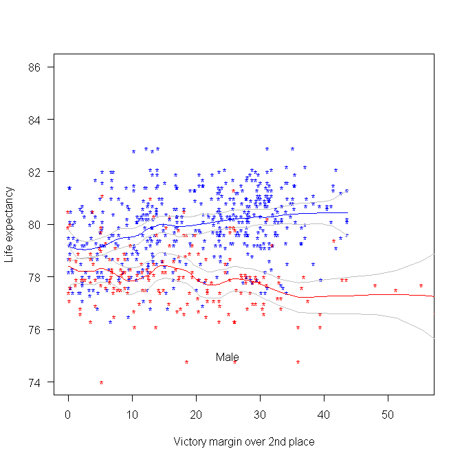
Rather than scrape the election data (added to my TODO list), I decided to recreate the plot and tidy up the associated analysis code; it’s now available via the CampaignLab Github repo

My interpretation of the difference in life-expectancy is that the Labour strongholds are in regions where there is (or once was) lots of heavy industry and mining; the kind of jobs where people don’t live long after retiring.

Offer of free analysis of your software engineering data

Derek Jones from The Shape of Code

Since the start of this year, I have been telling people that I willing to analyze their software engineering data for free, provided they are willing to make the data public; I also offer to anonymize the data for them, as part of the free service. Alternatively you could read this book, and do the analysis yourself.

What will you get out of me analyzing your data?

My aim is to find patterns of behavior that will be useful to you. What is useful to you? You have to be the judge of that. It is possible that I will not find anything useful, or perhaps any patterns at all; this does not happen very often. Over the last year I have found (what I think are useful) patterns in several hundred datasets, with one dataset that I am still scratching my head over it.

Data analysis is a two-way conversation. I find some patterns, and we chat about them, hopefully you will say one of them is useful, or point me in a related direction, or even a completely new direction; the process is iterative.

The requirement that an anonymized form of the data be made public is likely to significantly reduce the offers I receive.

There is another requirement that I don’t say much about: the data has to be interesting.

What makes software engineering data interesting, or at least interesting to me?

There has to be lots of it. How much is lots?

Well, that depends on the kind of data. Many kinds of measurements of source code are generally available by the truck load. Measurements relating to human involvement in software development are harder to come by, but becoming more common.

If somebody has a few thousand measurements of some development related software activity, I am very interested. However, depending on the topic, I might even be interested in a couple of dozen measurements.

Some measurements are very rare, and I would settle for as few as two measurements. For instance, multiple implementations of the same set of requirements provides information on system development variability; I was interested in five measurements of the lines of source in five distinct Pascal compilers for the same machine.

Effort estimation data used to be rare; published papers sometimes used to include a table containing the estimate/actual data, which was once gold-dust. These days I would probably only be interested if there were a few hundred estimates, but it would depend on what was being estimated.

If you have some software engineering data that you think I might be interested in, please email to tell me something about the data (and perhaps what you would like to know about it). I’m always open to a chat.

If we both agree that it’s worth looking at your data (I will ask you to confirm that you have the rights to make it public), then you send me the data and off we go.

Modeling visual studio C++ compile times

Derek Jones from The Shape of Code

Last week I spotted an interesting article on the compile-time performance of C++ compilers running under Microsoft Windows. The author had obviously put a lot of work into gathering the data, and had taken care to have multiple runs to reduce the impact of random effects (128 runs to be exact); but, as if often the case, the analysis of the data was lackluster. I posted a comment asking for the data, and a link was posted the next day :-)

The compilers benchmarked were: Visual Studio 2015, Visual Studio 2017 and clang 7.0.1; the compilers were configured to target: C++20, C++17, C++14, C++11, C++03, or C++98. The source code used was 100 system headers.

If we are interested in understanding the contribution of each component to overall compile-time, the obvious fist regression model to build is:

compile_time = header_x+compiler_y+language_z

where: header_x 
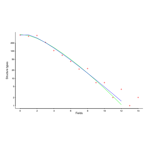
are the different headers, compiler_y the different compilers and language_z the different target languages. There might be some interaction between variables, so something more complicated was tried first; the final fitted model was (code+data):

compile_time = k+header_x+compiler_y+language_z+compiler_y*language_z

where k is a constant (the Intercept in R’s summary output). The following is a list of normalised numbers to plug into the equation (clang is the default compiler and C++03 the default language, and so do not appear in the list, the : symbol represents the multiplication; only a few of the 100 headers are listed, details are available):

                             Estimate Std. Error  t value Pr(>|t|)    
               (Intercept)                  headerany 
               1.000000000                0.051100398 
               headerarray             headerassert.h 
               0.522336397               -0.654056185 
...
            headerwctype.h            headerwindows.h 
              -0.648095154                1.304270250 
              compilerVS15               compilerVS17 
              -0.185795534               -0.114590143 
             languagec++11              languagec++14 
               0.032930014                0.156363433 
             languagec++17              languagec++20 
               0.192301727                0.184274629 
             languagec++98 compilerVS15:languagec++11 
               0.001149643               -0.058735591 
compilerVS17:languagec++11 compilerVS15:languagec++14 
              -0.038582437               -0.183708714 
compilerVS17:languagec++14 compilerVS15:languagec++17 
              -0.164031495                         NA 
compilerVS17:languagec++17 compilerVS15:languagec++20 
              -0.181591418                         NA 
compilerVS17:languagec++20 compilerVS15:languagec++98 
              -0.193587045                0.062414667 
compilerVS17:languagec++98 
               0.014558295 

As an example, the (normalised) time to compile wchar.h using VS15 with languagec++11 is:
1-0.514807638-0.183862162+0.033951731-0.059720131

Each component adds/substracts to/from the normalised mean.

Building this model didn’t take long. While waiting for the kettle to boil, I suddenly realised that an additive model was probably inappropriate for this problem; oops. Surely the contribution of each component was multiplicative, i.e., components have a percentage impact to performance.

A quick change to the form of the fitted model:

log(compile_time) = k+header_x+compiler_y+language_z+compiler_y*language_z

Taking the exponential of both side, the fitted equation becomes:

compile_time = e^{k}e^{header_x}e^{compiler_y}e^{language_z}e^{compiler_y*language_z}

The numbers, after taking the exponent, are:

               (Intercept)                  headerany 
              9.724619e+08               1.051756e+00 
...
            headerwctype.h            headerwindows.h 
              3.138361e-01               2.288970e+00 
              compilerVS15               compilerVS17 
              7.286951e-01               7.772886e-01 
             languagec++11              languagec++14 
              1.011743e+00               1.049049e+00 
             languagec++17              languagec++20 
              1.067557e+00               1.056677e+00 
             languagec++98 compilerVS15:languagec++11 
              1.003249e+00               9.735327e-01 
compilerVS17:languagec++11 compilerVS15:languagec++14 
              9.880285e-01               9.351416e-01 
compilerVS17:languagec++14 compilerVS15:languagec++17 
              9.501834e-01                         NA 
compilerVS17:languagec++17 compilerVS15:languagec++20 
              9.480678e-01                         NA 
compilerVS17:languagec++20 compilerVS15:languagec++98 
              9.402461e-01               1.058305e+00 
compilerVS17:languagec++98 
              1.001267e+00 

Taking the same example as above: wchar.h using VS15 with c++11. The compile-time (in cpu clock cycles) is:
9.724619e+08*3.138361e-01*7.286951e-01*1.011743e+00*9.735327e-01

Now each component causes a percentage change in the (mean) base value.

Both of these model explain over 90% of the variance in the data, but this is hardly surprising given they include so much detail.

In reality compile-time is driven by some combination of additive and multiplicative factors. Building a combined additive and multiplicative model is going to be like wrestling an octopus, and is left as an exercise for the reader :-)

Given a choice between these two models, I think the multiplicative model is probably closest to reality.

Teaching basic data analysis to programmers: summer internship

Derek Jones from The Shape of Code

Software engineering is one of the topics in this year’s summer internships being sponsored by R-Studio. The spec says: “Data Science Training for Software Engineers – Develop course materials to teach basic data analysis to programmers using software engineering problems and data sets.”

It’s good to see interest in data analysis of software engineering data start to gain traction.

What topics might basic data analysis for programmers include? I have written about statistical techniques that I think are useful in software engineering, but I don’t think this list would be regarded as basic. Techniques that are think are basic are:

  • a picture is worth a thousand words, so obviously visualization is a major topic,
  • building regression models is good for helping to understand what is going on.

Anything else? Well, I don’t know.

An alternative approach to teaching basic data analysis is to give examples of the kind of useful things it can be used to do. Software developers are fast learners, and given the motivation have the skills needed to find and learn techniques that they think are of use. In a basic course, I would put the emphasis on motivating developers to think that data analysis can help them do a better job.

I would NOT, repeat, not, include any material on machine learning. Software engineering data sets tend to be too small to obtain reliable results from machine learning, and I don’t want to encourage clueless button pushers.

What are the desirable skills in the summer intern? I would say that being able to write readable material is the most important, with statistical knowledge ranked second; the level of software engineering knowledge is unimportant. Data analysis tends to follow the same pattern whatever the subject; so it’s important to get somebody who knows about data analysis.

A social science major is the obvious demographic for this intern (they do lots of data analysis); the last people to consider are students majoring in a computing subject.

Choosing between two reasonably fitting probability distributions

Derek Jones from The Shape of Code

I sometimes go fishing for a probability distribution to fit some software engineering data I have. Why would I want to spend time fishing for a probability distribution?

Data comes from events that are driven by one or more processes. Researchers have studied the underlying patterns present in many processes and in some cases have been able to calculate which probability distribution matches the pattern of data that it generates. This approach starts with the characteristics of the processes and derives a probability distribution. Often I don’t really know anything about the characteristics of the processes that generated the data I am looking at (but I can often make what I like to think are intelligent guesses). If I can match the data with a probability distribution, I can use what is known about processes that generate this distribution to get some ideas about the kinds of processes that could have generated my data.

Around nine-months ago, I learned about the Conway–Maxwell–Poisson distribution (or COM-Poisson). This looked as-if it might find some use in fitting software engineering data, and I added it to my list of distributions to keep in mind. I saw that the R package COMPoissonReg supports the fitting of COM-Poisson distributions.

This week I came across one of the papers, about COM-Poisson, that I was reading nine-months ago, and decided to give it a go with some count-data I had.

The Poisson distribution involves count-data, i.e., non-negative integers. Lots of count-data samples are well described by a Poisson distribution, and it is one of the basic distributions supported by statistical packages. Processes described by a Poisson distribution are memory-less, in that the probability of an event occurring are independent of when previous events occurred. When there is a connection between events, the Poisson distribution is not such a good fit (depending on the strength of the connection between events).

While a process that generates count-data may not meet the requirements needed to be exactly described by a Poisson distribution, the behavior may be close enough to give good-enough results. R supports a quasipoisson distribution to help handle the ‘near-misses’.

Sometimes count-data has a distribution that looks nothing like a Poisson. The Negative-binomial distribution is the obvious next choice to try (this can be viewed as a combination of different Poisson distributions; another combination is the Poisson inverse gaussian distribution).

The plot below (from a paper analyzing usage of record data structures in Racket; Tobias Pape kindly sent me the data) shows the number of Racket structure types that contain a given number of fields (red pluses), along with lines showing fitted Negative binomial and COM-Poisson distributions (code+data):

Number of Racket structure types containing a given number of fields.

I’m interested in understanding the processes that are generating the data, and having two distributions do such a reasonable job of fitting the data has given me more possible distinct explanations for what is going on than I wanted (if I were interested in prediction, then either distribution looks like it would do a good-enough job).

What are the characteristics of the processes that generate data having each of the distributions?

  • A Negative binomial can be viewed as a combination of Poisson distributions (the combination having a Gamma distribution). We could create a story around multiple processes being responsible for the pattern seen, with each of these processes having the impact of a Poisson distribution. Sounds plausible.
  • A COM-Poisson distribution can be viewed as a Poisson distribution which is length dependent. We could create a story around the probability of a field being added to a structure type being dependent on the number of existing fields it contains. Sounds plausible (it’s a slightly different idea from preferential attachment).

When fitting a distribution to data, I usually go with the ‘brand-name’ distributions (i.e., the one with most name recognition, provided it matches well enough; brand names are an easier sell then the less well known names).

The Negative binomial distribution is the brand-name here. I had not heard of the COM-Poisson distribution until nine-months ago.

Perhaps the authors of the Racket analysis paper will come up with a theory that prefers one of these distributions, or even suggests another one.

Readers of my evidence-based software engineering book need to be aware of my brand-name preference in some of the data fitting that occurs.

Wanted: 99 effort estimation datasets

Derek Jones from The Shape of Code

Every now and again, I stumble upon a really interesting dataset. Previously, when this happened I wrote an extensive blog post; but the SiP dataset was just too big and too detailed, it called out for a more expansive treatment.

How big is the SiP effort estimation dataset? It contains 10,100 unique task estimates, from ten years of commercial development using Agile. That’s around two orders of magnitude larger than other, current, public effort datasets.

How detailed is the SiP effort estimation dataset? It contains the (anonymized) identity of the 22 developers making the estimates, for one of 20 project codes, dates, plus various associated items. Other effort estimation datasets usually just contain values for estimated effort and actual effort.

Data analysis is a conversation between the person doing the analysis and the person(s) with knowledge of the application domain from which the data came. The aim is to discover information that is of practical use to the people working in the application domain.

I suggested to Stephen Cullum (the person I got talking to at a workshop, a director of Software in Partnership Ltd, and supplier of data) that we write a paper having the form of a conversation about the data; he bravely agreed.

The result is now available: A conversation around the analysis of the SiP effort estimation dataset.

What next?

I’m looking forward to seeing what other people do with the SiP dataset. There are surely other patterns waiting to be discovered, and what about building a simulation model based on the charcteristics of this data?

Turning software engineering into an evidence-based disciple requires a lot more data; I plan to go looking for more large datasets.

Software engineering researchers are a remarkable unambitious bunch of people. The SiP dataset should be viewed as the first of 100 such datasets. With 100 datasets we can start to draw general, believable conclusions about the processes involved in software effort estimation.

Readers, today is the day you start asking managers to make any software engineering data they have publicly available. Yes, it can be anonymized (I am willing to do that for people who are looking to release data). Yes, ‘old’ data is useful (data from the 1980s could have an interesting story to tell; SiP runs from 2004-2014). Yes, I will analyze any interesting data that is made public for free.

Ask, and you shall receive.

Changes in the shape of code during the twenties?

Derek Jones from The Shape of Code

At the end of 2009 I made two predictions for the next decade; Chinese and Indian developers having a major impact on the shape of code (ok, still waiting for this to happen), and scripting languages playing a significant role (got that one right, but then they were already playing a large role).

Since this blog has just entered its second decade, I will bring the next decade’s predictions forward a year.

I don’t see any new major customer ecosystems appearing. Ecosystems are the drivers of software development, and no new ecosystems has several consequences, including:

  • No major new languages: Creating a language is a vanity endeavor. Vanity project can take off if they are in the right place at the right time. New ecosystems provide opportunities for new languages to become widely used by being in at the start and growing with the ecosystem. There is another opportunity locus; it is fashionable for companies that see themselves as thought-leaders to have their own language, e.g., Google, Apple, and Mozilla. Invent your language at the right time, while working for a thought-leader company and your language could become well-known enough to take-off.

    I don’t see any major new ecosystems appearing and all the likely companies already have their own language.

    Any new language also faces the problem of not having a large collection packages.

  • Software will be more thoroughly tested: When an ecosystem is new, the incentives drive early and frequent releases (to build a customer base); software just has to be good enough. Once a product is established, companies can invest in addressing issues that customers find annoying, like faulty behavior; the incentive change results in more testing.

    There are other forces at work around testing. Companies are experiencing some very expensive faults (testing may be expensive, but not testing may be more expensive) and automatic test generation is becoming commercially usable (i.e., the cost of some kinds of testing is decreasing).

The evolution of widely used languages.

  • I think Fortran and C will have new features added, with relatively little fuss, and will quietly continue to be widely used (to the dismay of the fashionista).
  • There is a strong expectation that C++ and Java should continue to evolve:

    • I expect the ISO C++ work to implode, because there are too many people pulling in too many directions. It makes sense for the gcc and llvm teams to cooperate in taking C++ in a direction that satisfies developers’ needs, rather than the needs of bored consultants. What are Microsoft’s views? They only have their own compiler for strategic reasons (they make little if any profit selling compilers, compilers are an unnecessary drain on management time; who cares what happens to the language).
    • It is going to be interesting watching the impact of Oracle’s move to charging for runtimes. I have no idea what might happen to Java.

In terms of code volume, the future surely has to be scripting languages, and in particular Python, Javascript and PHP. Ten years from now, will there be a widely used, single language? People have been predicting, for many years, that web languages will take over the world; perhaps there will be a sudden switch and I will see that the choice is obvious.

Moore’s law is now dead, which means researchers are going to have to look for completely new techniques for building logic gates. If photonic computers happen, then ternary notation may reappear again (it was used in at least one early Russian computer); I’m not holding my breath for this to occur.

Foundations for Evidence-Based Policymaking Act of 2017

Derek Jones from The Shape of Code

The Foundations for Evidence-Based Policymaking Act of 2017 was enacted by the US Congress on 21st December.

A variety of US Federal agencies are responsible for ensuring the safety of US citizens, in some cases this safety is dependent on the behavior of software. The FDA is responsible for medical device safety and the FAA publishes various software safety handbooks relating to aviation (the Department of transportation has a wider remit).

Where do people go to learn about the evidence for software related issues?

The book: Evidence-based software engineering: based on the publicly available evidence sounds like a good place to start.

Quickly skimming this (currently draft) book shows that no public evidence is available on lots of issues. Oops.

Another issue is the evidence pointing to some suggested practices being at best useless and sometimes fraudulent, e.g., McCabe’s cyclomatic complexity metric.

The initial impact of evidence-based policymaking will be companies pushing back against pointless government requirements, in particular requirements that cost money to implement. In some cases this is a good, e.g., no more charades about software being more testable because its code has a low McCable complexity.

In the slightly longer term, people are going to have to get serious about collecting and analyzing software related evidence.

The Open, Public, Electronic, and Necessary Government Data Act or the OPEN Government Data Act (which is about to become law) will be a big help in obtaining evidence. I think there is a lot of software related data sitting on disks and tapes, waiting to be analysed (NASA appears to have loads to data that they have down almost nothing with, including not making it publicly available).

Interesting times ahead.

Distorting the input profile, to stress test a program

Derek Jones from The Shape of Code

A fault is experienced in software when there is a mistake in the code, and a program is fed the input values needed for this mistake to generate faulty behavior.

There is suggestive evidence that the distribution of coding mistakes and inputs generating fault experiences both have an influence of fault discovery.

How might these coding mistakes be found?

Testing is one technique, it involves feeding inputs into a program and checking the resulting behavior. What are ‘good’ input values, i.e., values most likely to discover problems? There is no shortage of advice for manually writing tests, suggesting how to select input values, but automatic generation of inputs is often somewhat random (relying on quantity over quality).

Probabilistic grammar driven test generators are trivial to implement. The hard part is tuning the rules and the probability of them being applied.

In most situations an important design aim, when creating a grammar, is to have one rule for each construct, e.g., all arithmetic, logical and boolean expressions are handled by a single expression rule. When generating tests, it does not always make sense to follow this rule; for instance, logical and boolean expressions are much more common in conditional expressions (e.g., controlling an if-statement), than other contexts (e.g., assignment). If the intent is to mimic typical user input values, then the probability of generating a particular kind of binary operator needs to be context dependent; this might be done by having context dependent rules or by switching the selection probabilities by context.

Given a grammar for a program’s input (e.g., the language grammar used by a compiler), decisions have to be made about the probability of each rule triggering. One way of obtaining realistic values is to parse existing input, counting the number of times each rule triggers. Manually instrumenting a grammar to do this is a tedious process, but tool support is now available.

Once a grammar has been instrumented with probabilities, it can be used to generate tests.

Probabilities based on existing input will have the characteristics of that input. A recent paper on this topic (which prompted this post) suggests inverting rule probabilities, so that common becomes rare and vice versa; the idea is that this will maximise the likelihood of a fault being experienced (the assumption is that rarely occurring input will exercise rarely executed code, and such code is more likely to contain mistakes than frequently executed code).

I would go along with the assumption about rarely executed code having a greater probability of containing a mistake, but I don’t think this is the best test generation strategy.

Companies are only interested in fixing the coding mistakes that are likely to result of a fault being experienced by a customer. It is a waste of resources to fix a mistake that will never result in a fault experienced by a customer.

What input is likely to interact with coding mistakes to be the root cause of faults experienced by a customer? I have no good answer to this question. But, given there are customer input contains patterns (at least in the world of source code, and I’m told in other application domains), I would generate test cases that are very similar to existing input, but with one sub-characteristic changed.

In the academic world the incentive is to publish papers reporting loads-of-faults-found, the more the merrier. Papers reporting only a few faults are obviously using inferior techniques. I understand this incentive, but fixing problems costs money and companies want a customer oriented rationale before they will invest in fixing problems before they are reported.

The availability of tools that automate the profiling of a program’s existing input, followed by the generation of input having slightly, or very, different characteristics make it easier to answer some very tough questions about program behavior.

Growth of conditional complexity with file size

Derek Jones from The Shape of Code

Conditional statements are a fundamental constituent of programs. Conditions are driven by the requirements of the problem being solved, e.g., if the water level is below the minimum, then add more water. As the problem being solved gets more complicated, dependencies between subproblems grow, requiring an increasing number of situations to be checked.

A condition contains one or more clauses, e.g., a single clause in: if (a==1), and two clauses in: if ((x==y) && (z==3)); a condition also appears as the termination test in a for-loop.

How many conditions containing one clause will a 10,000 line program contain? What will be the distribution of the number of clauses in conditions?

A while back I read a paper studying this problem (“What to expect of predicates: An empirical analysis of predicates in real world programs”; Google currently not finding a copy online, grrr, you will have to hassle the first author: durelli@icmc.usp.br, or perhaps it will get added to a list of favorite publications {be nice, they did publish some very interesting data}) it contained a table of numbers and yesterday my analysis of the data revealed a surprising pattern.

The data consists of SLOC, number of files and number of conditions containing a given number of clauses, for 63 Java programs. The following plot shows percentage of conditionals containing a given number of clauses (code+data):

Percentage of conditions containing a given number of clauses in 63 large Java programs.

The fitted equation, for the number of conditionals containing a given number of clauses, is:

conditions = 3*slen^pred e^{10-10pred-1.8 10^{-5}avlen^2}

where: slen={SLOC}/{sqrt{Number of Files}} 
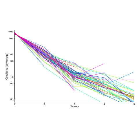
(the coefficient for the fitted regression model is 0.56, but square-root is easier to remember), avlen={SLOC}/{Number of Files}, and pred is the number of clauses.

The fitted regression model is not as good when slen or avlen is always used.

This equation is an emergent property of the code; simply merging files to increase the average length will not change the distribution of clauses in conditionals.

When slen = e^{10} = 22,026, all conditionals contain the same number of clauses, off to infinity. For the 63 Java programs, the mean slen was 2,625, maximum 11,710, and minimum 172.

I was expecting SLOC to have an impact, but was not expecting number of files to be involved.

What grows with SLOC? Number of global variables and number of dependencies. There are more things available to be checked in larger programs, and an increase in dependencies creates the need to perform more checks. Also, larger programs are likely to contain more special cases, which are likely to involve checking both general and specific values (i.e., more clauses in conditionals); ok, this second sentence is a bit more arm-wavy than the first. The prediction here is that the percentage of global variables appearing in conditions increases with SLOC.

Chopping stuff up into separate files has a moderating effect. Since I did not expect this, I don’t have much else to say.

This model explains 74% of the variance in the data (impressive, if I say so myself). What other factors might be involved? Depth of nesting would be my top candidate.

Removing non-if-statement related conditionals from the count would help clarify things (I don’t expect loop-controlling conditions to be related to amount of code).

Two interesting data-sets in one week, with 10-days still to go until Christmas :-)