regression model – ACCU World of Code

Derek Jones from The Shape of Code

Sorting and searching are probably the most widely performed operations in computing; they are extensively covered in volume 3 of The Art of Computer Programming. Algorithm performance is influence by the characteristics of the processor on which it runs, and the size of the processor cache(s) has a significant impact on performance.

A study by Khuong and Morin investigated the performance of various search algorithms on 46 different processors. Khuong kindly sent me a copy of the raw data; the study webpage includes lots of plots.

The performance comparison involved 46 processors (mostly Intel x86 compatible cpus, plus a few ARM cpus) times 3 array datatypes times 81 array sizes times 28 search algorithms. First a 32/64/128-bit array of unsigned integers containing N elements was initialized with known values. The benchmark iterated 2-million times around randomly selecting one of the known values, and then searching for it using the algorithm under test. The time taken to iterate 2-million times was recorded. This was repeated for the 81 values of N, up to 63,095,734, on each of the 46 processors.

The plot below shows the results of running each algorithm benchmarked (colored lines) on an Intel Atom D2700 @ 2.13GHz, for 32-bit array elements; the kink in the lines occur roughly at the point where the size of the array exceeds the cache size (all code+data):

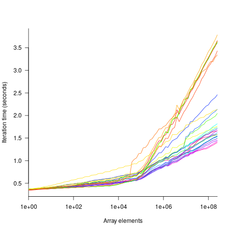
What is the most effective way of analyzing the measurements to produce consistent results?

One approach is to build two regression models, one for the measurements before the cache ‘kink’ and one for the measurements after this kink. By adding in a dummy variable at the kink-point, it is possible to merge these two models into one model. The problem with this approach is that the kink-point has to be chosen in advance. The plot shows that the performance kink occurs before the array size exceeds the cache size; other variables are using up some of the cache storage.

This approach requires fitting 46*3=138 models (I think the algorithm used can be integrated into the model).

If data from lots of processors is to be fitted, or the three datatypes handled, an automatic way of picking where the first regression model should end, and where the second regression model should start is needed.

Regression discontinuity design looks like it might be applicable; treating the point where the array size exceeds the cache size as the discontinuity. Traditionally discontinuity designs assume a sharp discontinuity, which is not the case for these benchmarks (R’s rdd package worked for one algorithm, one datatype running on one processor); the more recent continuity-based approach supports a transition interval before/after the discontinuity. The R package rdrobust supports a continued-based approach, but seems to expect the discontinuity to be a change of intercept, rather than a change of slope (or rather, I could not figure out how to get it to model a just change of slope; suggestions welcome).

Another approach is to use segmented regression, i.e., one of more distinct lines. The package segmented supports fitting this kind of model, and does estimate what they call the breakpoint (the user has to provide a first estimate).

I managed to fit a segmented model that included all the algorithms for 32-bit data, running on one processor (code+data). Looking at the fitted model I am not hopeful that adding data from more than one processor would produce something that contained useful information. I suspect that there are enough irregular behaviors in the benchmark runs to throw off fitting quality.

I’m always asking for more data, and now I have more data than I know how to analyze in a way that does not require me to build 100+ models

Suggestions welcome.

Derek Jones from The Shape of Code

Running an experiment is very time-consuming. I am always surprised that people put so much effort into gathering the data and then spend so little effort analyzing it.

The Computer Language Benchmarks Game looks like a fun benchmark; it compares the performance of 27 languages using various toy benchmarks (they could not be said to be representative of real programs). And, yes, lots of boxplots and tables of numbers; great eye-candy, but what do they all mean?

The authors, like good experimentalists, make all their data available. So, what analysis should they have done?

A regression model is the obvious choice and the following three lines of R (four lines if you could the blank line) build one, providing lots of interesting performance information:

cl=read.csv("Computer-Language_u64q.csv.bz2", as.is=TRUE)

cl_mod=glm(log(cpu.s.) ~ name+lang, data=cl)
summary(cl_mod)

The following is a cut down version of the output from the call to summary, which summarizes the model built by the call to glm.

                    Estimate Std. Error t value Pr(>|t|)    
(Intercept)         1.299246   0.176825   7.348 2.28e-13 ***
namechameneosredux  0.499162   0.149960   3.329 0.000878 ***
namefannkuchredux   1.407449   0.111391  12.635  < 2e-16 ***
namefasta           0.002456   0.106468   0.023 0.981595    
namemeteor         -2.083929   0.150525 -13.844  < 2e-16 ***

langclojure         1.209892   0.208456   5.804 6.79e-09 ***
langcsharpcore      0.524843   0.185627   2.827 0.004708 ** 
langdart            1.039288   0.248837   4.177 3.00e-05 ***
langgcc            -0.297268   0.187818  -1.583 0.113531 
langocaml          -0.892398   0.232203  -3.843 0.000123 *** 
  
    Null deviance: 29610  on 6283  degrees of freedom
Residual deviance: 22120  on 6238  degrees of freedom

What do all these numbers mean?

We start with glm's first argument, which is a specification of the regression model we are trying to fit: log(cpu.s.) ~ name+lang

cpu.s. is cpu time, name is the name of the program and lang is the language. I found these by looking at the column names in the data file. There are other columns in the data, but I am running in quick & simple mode. As a first stab, I though cpu time would depend on the program and language. Why take the log of the cpu time? Well, the model fitted using cpu time was very poor; the values range over several orders of magnitude and logarithms are a way of compressing this range (and the fitted model was much better).

The model fitted is:

$cpu.s. = e^{Intercept+name+prog}$ , or $cpu.s. = e^{Intercept}*e^{name}*e^{prog}$

Plugging in some numbers, to predict the cpu time used by say the program chameneosredux written in the language clojure, we get: $cpu.s. = e^{1.3}*e^{0.5}*e^{1.2}=20.1$ (values taken from the first column of numbers above).

This model assumes there is no interaction between program and language. In practice some languages might perform better/worse on some programs. Changing the first argument of glm to: log(cpu.s.) ~ name*lang, adds an interaction term, which does produce a better fitting model (but it's too complicated for a short blog post; another option is to build a mixed-model by using lmer from the lme4 package).

We can compare the relative cpu time used by different languages. The multiplication factor for clojure is $e^{1.2}=3.3$ , while for ocaml it is $e^{-0.9}=0.4$ . So clojure consumes 8.2 times as much cpu time as ocaml.

How accurate are these values, from the fitted regression model?

The second column of numbers in the summary output lists the estimated standard deviation of the values in the first column. So the clojure value is actually $e^{1.2 pm (0.2*1.96)}$ , i.e., between 2.2 and 4.9 (the multiplication by 1.96 is used to give a 95% confidence interval); the ocaml values are $e^{-0.9 pm (0.2*1.96)}$ , between 0.3 and 0.6.

The fourth column of numbers is the p-value for the fitted parameter. A value of lower than 0.05 is a common criteria, so there are question marks over the fit for the program fasta and language gcc. In fact many of the compiled languages have high p-values, perhaps they ran so fast that a large percentage of start-up/close-down time got included in their numbers. Something for the people running the benchmark to investigate.

Isn't it easy to get interesting numbers by building a regression model? It took me 10 minutes, ok I spend a lot of time fitting models. After spending many hours/days gathering data, spending a little more time learning to build simple regression models is well worth the effort.

Category: regression model

Fitting discontinuous data from disparate sources

Building a regression model is easy and informative