Derek Jones from The Shape of Code
I sometimes go fishing for a probability distribution to fit some software engineering data I have. Why would I want to spend time fishing for a probability distribution?
Data comes from events that are driven by one or more processes. Researchers have studied the underlying patterns present in many processes and in some cases have been able to calculate which probability distribution matches the pattern of data that it generates. This approach starts with the characteristics of the processes and derives a probability distribution. Often I don’t really know anything about the characteristics of the processes that generated the data I am looking at (but I can often make what I like to think are intelligent guesses). If I can match the data with a probability distribution, I can use what is known about processes that generate this distribution to get some ideas about the kinds of processes that could have generated my data.
Around nine-months ago, I learned about the Conway–Maxwell–Poisson distribution (or COM-Poisson). This looked as-if it might find some use in fitting software engineering data, and I added it to my list of distributions to keep in mind. I saw that the R package COMPoissonReg supports the fitting of COM-Poisson distributions.
This week I came across one of the papers, about COM-Poisson, that I was reading nine-months ago, and decided to give it a go with some count-data I had.
The Poisson distribution involves count-data, i.e., non-negative integers. Lots of count-data samples are well described by a Poisson distribution, and it is one of the basic distributions supported by statistical packages. Processes described by a Poisson distribution are memory-less, in that the probability of an event occurring are independent of when previous events occurred. When there is a connection between events, the Poisson distribution is not such a good fit (depending on the strength of the connection between events).
While a process that generates count-data may not meet the requirements needed to be exactly described by a Poisson distribution, the behavior may be close enough to give good-enough results. R supports a quasipoisson distribution to help handle the ‘near-misses’.
Sometimes count-data has a distribution that looks nothing like a Poisson. The Negative-binomial distribution is the obvious next choice to try (this can be viewed as a combination of different Poisson distributions; another combination is the Poisson inverse gaussian distribution).
The plot below (from a paper analyzing usage of record data structures in Racket; Tobias Pape kindly sent me the data) shows the number of Racket structure types that contain a given number of fields (red pluses), along with lines showing fitted Negative binomial and COM-Poisson distributions (code+data):
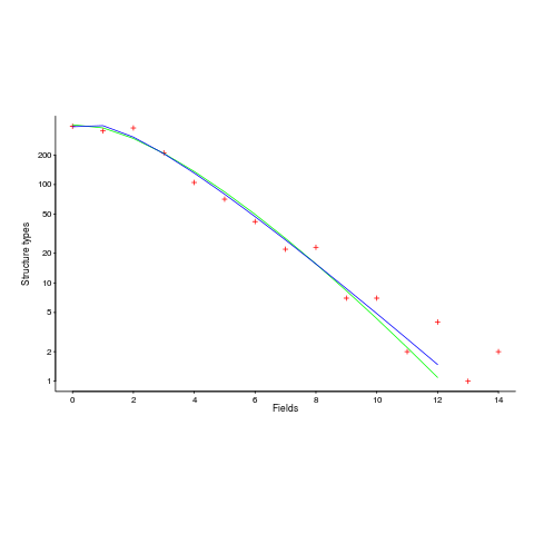
I’m interested in understanding the processes that are generating the data, and having two distributions do such a reasonable job of fitting the data has given me more possible distinct explanations for what is going on than I wanted (if I were interested in prediction, then either distribution looks like it would do a good-enough job).
What are the characteristics of the processes that generate data having each of the distributions?
- A Negative binomial can be viewed as a combination of Poisson distributions (the combination having a Gamma distribution). We could create a story around multiple processes being responsible for the pattern seen, with each of these processes having the impact of a Poisson distribution. Sounds plausible.
- A COM-Poisson distribution can be viewed as a Poisson distribution which is length dependent. We could create a story around the probability of a field being added to a structure type being dependent on the number of existing fields it contains. Sounds plausible (it’s a slightly different idea from preferential attachment).
When fitting a distribution to data, I usually go with the ‘brand-name’ distributions (i.e., the one with most name recognition, provided it matches well enough; brand names are an easier sell then the less well known names).
The Negative binomial distribution is the brand-name here. I had not heard of the COM-Poisson distribution until nine-months ago.
Perhaps the authors of the Racket analysis paper will come up with a theory that prefers one of these distributions, or even suggests another one.
Readers of my evidence-based software engineering book need to be aware of my brand-name preference in some of the data fitting that occurs.