Some human biases in conditional reasoning

Derek Jones from The Shape of Code

Tracking down coding mistakes is a common developer activity (for which training is rarely provided).

Debugging code involves reasoning about differences between the actual and expected output produced by particular program input. The goal is to figure out the coding mistake, or at least narrow down the portion of code likely to contain the mistake.

Interest in human reasoning dates back to at least ancient Greece, e.g., Aristotle and his syllogisms. The study of the psychology of reasoning is very recent; the field was essentially kick-started in 1966 by the surprising results of the Wason selection task.

Debugging involves a form of deductive reasoning known as conditional reasoning. The simplest form of conditional reasoning involves an input that can take one of two states, along with an output that can take one of two states. Using coding notation, this might be written as:

    if (p) then q       if (p) then !q
    if (!p) then q      if (!p) then !q

The notation used by the researchers who run these studies is a 2×2 contingency table (or conditional matrix):

          OUTPUT
          1    0
   
      1   A    B
INPUT
      0   C    D

where: A, B, C, and D are the number of occurrences of each case; in code notation, p is the input and q the output.

The fertilizer-plant problem is an example of the kind of scenario subjects answer questions about in studies. Subjects are told that a horticultural laboratory is testing the effectiveness of 31 fertilizers on the flowering of plants; they are told the number of plants that flowered when given fertilizer (A), the number that did not flower when given fertilizer (B), the number that flowered when not given fertilizer (C), and the number that did not flower when not given any fertilizer (D). They are then asked to evaluate the effectiveness of the fertilizer on plant flowering. After the experiment, subjects are asked about any strategies they used to make judgments.

Needless to say, subjects do not make use of the available information in a way that researchers consider to be optimal, e.g., Allan’s Delta p index Delta p=P(A vert C)-P(B vert D)=A/{A+B}-C/{C+D} (sorry about the double, vert, rather than single, vertical lines).

What do we know after 40+ years of active research into this basic form of conditional reasoning?

The results consistently find, for this and other problems, that the information A is given more weight than B, which is given by weight than C, which is given more weight than D.

That information provided by A and B is given more weight than C and D is an example of a positive test strategy, a well-known human characteristic.

Various models have been proposed to ‘explain’ the relative ordering of information weighting: w(A)>w(B) > w(C) > w(D)” title=”w(A)>w(B) > w(C) > w(D)”/><a href=
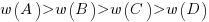
, e.g., that subjects have a bias towards sufficiency information compared to necessary information.

Subjects do not always analyse separate contingency tables in isolation. The term blocking is given to the situation where the predictive strength of one input is influenced by the predictive strength of another input (this process is sometimes known as the cue competition effect). Debugging is an evolutionary process, often involving multiple test inputs. I’m sure readers will be familiar with the situation where the output behavior from one input motivates a misinterpretation of the behaviour produced by a different input.

The use of logical inference is a commonly used approach to the debugging process (my suggestions that a statistical approach may at times be more effective tend to attract odd looks). Early studies of contingency reasoning were dominated by statistical models, with inferential models appearing later.

Debugging also involves causal reasoning, i.e., searching for the coding mistake that is causing the current output to be different from that expected. False beliefs about causal relationships can be a huge waste of developer time, and research on the illusion of causality investigates, among other things, how human interpretation of the information contained in contingency tables can be ‘de-biased’.

The apparently simple problem of human conditional reasoning over two variables, each having two states, has proven to be a surprisingly difficult to model. It is tempting to think that the performance of professional software developers would be closer to the ideal, compared to the typical experimental subject (e.g., psychology undergraduates or Mturk workers), but I’m not sure whether I would put money on it.

A study of deceit when reporting information in a known context

Derek Jones from The Shape of Code

A variety of conflicting factors intrude when attempting to form an impartial estimate of the resources needed to perform a task. The customer/manager, asking for the estimate wants to hear a low value, creating business/social pressure to underestimate; overestimating increases the likelihood of completing the task within budget.

A study by Oey, Schachner and Vul investigated the strategic reasoning for deception/lying in a two-person game.

A game involved a Sender and Receiver, with the two players alternating between the roles. The game started with both subjects seeing a picture of a box containing red and blue marbles (the percentage of red marbles was either 20%, 50%, or 80%). Ten marbles were randomly selected from this ‘box’, and shown to the Sender. The Sender was asked to report to the Receiver the number of red marbles appearing in the random selection, K_{report} (there was an incentive to report higher/lower, and punishment for being caught being inaccurate). The Receiver could accept or reject the number of red balls reported by the Sender. In the actual experiment, unknown to the human subjects, one of every game’s subject pair was always played by a computer. Every subject played 100 games.

In the inflate condition: If the Receiver accepted the report, the Sender gained K_{report} points, and the Receiver gained 10-K_{report} points.

If the Receiver rejected the report, then:

  • if the Sender’s report was accurate (i.e.,K_{report} == K_{actual}), the Sender gained K_{report} points, and the Receiver gained 10-K_{report}-5 points (i.e., a -5 point penalty),
  • if the Sender’s report was not accurate, the Receiver gained 5 points, and the Sender lost 5 points.

In the deflate condition: The points awarded to the Sender was based on the number of blue balls in the sample, and the points awarded to the Received was based on the number of red balls in the sample (i.e., the Sender had in incentive to report fewer red balls).

The plot below shows the mean rate of deceit (i.e., the fraction of a subject’s reports where K_{actual} < K_{report}
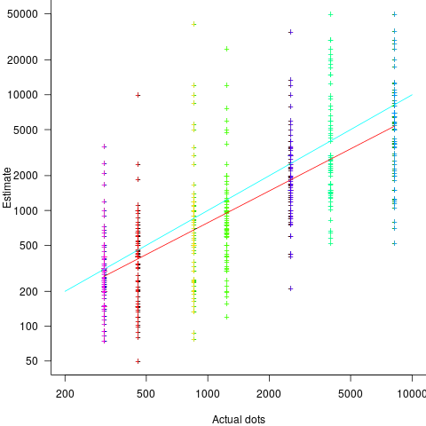
, averaged over all 116 subject’s mean) for a given number of red marbles actually seen by the Sender; vertical lines show one standard deviation, calculated over the mean of all subjects (code+data):

Mean rate of deceit for each number of red marbles seen, with bars showing standard deviation.

Subjects have some idea of the percentage of red/blue balls, and are aware that their opponent has a similar idea.

The wide variation in the fraction of reports where a subject reported a value greater than the number of marbles seen, is likely caused by variation in subject level of risk aversion. Some subjects may have decided to reduce effort by always accurately reporting, while others may have tried to see how much they could get away with.

The wide variation is particularly noticeable in the case of a box containing 80% red. If a Sender’s random selection contains few reds, then the Sender can feel confident reporting to have seen more.

The general pattern shows subjects being more willing to increase the reported number when they are supplied with few.

There is a distinct change of behavior when half of the sample contains more than five red marbles. In this situation, subjects may be happy to have been dealt a good hand, and are less inclined to risk losing 5-points for less gain.

Estimating involves considering more factors than the actual resources likely to be needed to implement the task; the use of round numbers is one example. This study is one of few experimental investigations of numeric related deception. The use of students having unknown motivation is far from ideal, but they are better than nothing.

When estimating in a team context, there is an opportunity to learn about the expectations of others and the consequences of over/under estimating. An issue for another study 🙂

Estimating quantities from several hundred to several thousand

Derek Jones from The Shape of Code

How much influence do anchoring and financial incentives have on estimation accuracy?

Anchoring is a cognitive bias which occurs when a decision is influenced by irrelevant information. For instance, a study by John Horton asked 196 subjects to estimate the number of dots in a displayed image, but before providing their estimate subjects had to specify whether they thought the number of dots was higher/lower than a number also displayed on-screen (this was randomly generated for each subject).

How many dots do you estimate appear in the plot below?

Image containing 500 dots.

Estimates are often round numbers, and 46% of dot estimates had the form of a round number. The plot below shows the anchor value seen by each subject and their corresponding estimate of the number of dots (the image always contained five hundred dots, like the one above), with round number estimates in same color rows (e.g., 250, 300, 500, 600; code+data):

Anchor value seen by a subject and corresponding estimate of number of dots.

How much influence does the anchor value have on the estimated number of dots?

One way of measuring the anchor’s influence is to model the estimate based on the anchor value. The fitted regression equation Estimate=54*Anchor^{0.33} 
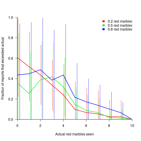
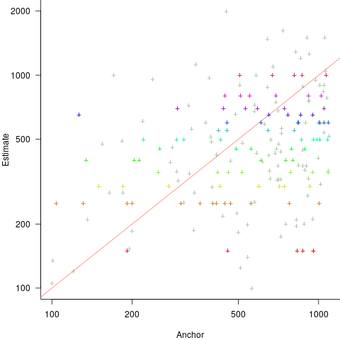
explains 11% of the variance in the data. If the higher/lower choice is included the model, 44% of the variance is explained; higher equation is: Estimate=169+1.1*Anchor and lower equation is: Estimate=169+0.36*Anchor (a multiplicative model has a similar goodness of fit), i.e., the anchor has three-times the impact when it is thought to be an underestimate.

How much would estimation accuracy improve if subjects’ were given the option of being rewarded for more accurate answers, and no anchor is present?

A second experiment offered subjects the choice of either an unconditional payment of $2.50 or a payment of $5.00 if their answer was in the top 50% of estimates made (labelled as the risk condition).

The 196 subjects saw up to seven images (65 only saw one), with the number of dots varying from 310 to 8,200. The plot below shows actual number of dots against estimated dots, for all subjects; blue/green line shows Estimate == Actual, and red line shows the fitted regression model Estimate approx Actual^{0.9} (code+data):

Actual and estimated number of dots in image seen by subjects.

The variance in the estimated number of dots is very high and increases with increasing actual dot count, however, this behavior is consistent with the increasing variance seen for images containing under 100 dots.

Estimates were not more accurate in those cases where subjects chose the risk payment option. This is not surprising, performance improvements require feedback, and subjects were not given any feedback on the accuracy of their estimates.

Of the 86 subjects estimating dots in three or more images, 44% always estimated low and 16% always high. Subjects always estimating low/high also occurs in software task estimates.

Estimation patterns previously discussed on this blog have involved estimated values below 100. This post has investigated patterns in estimates ranging from several hundred to several thousand. Patterns seen include extensive use of round numbers and increasing estimate variance with increasing actual value; all seen in previous posts.

How useful are automatically generated compiler tests?

Derek Jones from The Shape of Code

Over the last decade, testing compilers using automatically generated source code has been a popular research topic (for those working in the compiler field; Csmith kicked off this interest). Compilers are large complicated programs, and they will always contain mistakes that lead to faults being experienced. Previous posts of mine have raised two issues on the use of automatically generated tests: a financial issue (i.e., fixing reported faults costs money {most of the work on gcc and llvm is done by people working for large companies}, and is intended to benefit users not researchers seeking bragging rights for their latest paper), and applicability issue (i.e., human written code has particular characteristics and unless automatically generated code has very similar characteristics the mistakes it finds are unlikely to commonly occur in practice).

My claim that mistakes in compilers found by automatically generated code are unlikely to be the kind of mistakes that often lead to a fault in the compilation of human written code is based on the observations (I don’t have any experimental evidence): the characteristics of automatically generated source is very different from human written code (I know this from measurements of lots of code), and this difference results in parts of the compiler that are infrequently executed by human written code being more frequently executed (increasing the likelihood of a mistake being uncovered; an observation based on my years working on compilers).

An interesting new paper, Compiler Fuzzing: How Much Does It Matter?, investigated the extent to which fault experiences produced by automatically generated source are representative of fault experiences produced by human written code. The first author of the paper, Michaël Marcozzi, gave a talk about this work at the Papers We Love workshop last Sunday (videos available).

The question was attacked head on. The researchers instrumented the code in the LLVM compiler that was modified to fix 45 reported faults (27 from four fuzzing tools, 10 from human written code, and 8 from a formal verifier); the following is an example of instrumented code:

warn ("Fixing patch reached");
if (Not.isPowerOf2()) {
   if (!(C-> getValue().isPowerOf2()  // Check needed to fix fault
         && Not != C->getValue())) {
      warn("Fault possibly triggered");
   } else { /* CODE TRANSFORMATION */ } } // Original, unfixed code

The instrumented compiler was used to build 309 Debian packages (around 10 million lines of C/C++). The output from the builds were (possibly miscompiled) built versions of the packages, and log files (from which information could be extracted on the number of times the fixing patches were reached, and the number of cases where the check needed to fix the fault was triggered).

Each built package was then checked using its respective test suite; a package built from miscompiled code may successfully pass its test suite.

A bitwise compare was run on the program executables generated by the unfixed and fixed compilers.

The following (taken from Marcozzi’s slides) shows the percentage of packages where the fixing patch was reached during the build, the percentages of packages where code added to fix a fault was triggered, the percentage where a different binary was generated, and the percentages of packages where a failure was detected when running each package’s tests (0.01% is one failure):

Percentage of packages where patched code was reached during builds, and packages with failing tests.

The takeaway from the above figure is that many packages are affected by the coding mistakes that have been fixed, but that most package test suites are not affected by the miscompilations.

To find out whether there is a difference, in terms of impact on Debian packages, between faults reported in human and automatically generated code, we need to compare number of occurrences of “Fault possibly triggered”. The table below shows the break-down by the detector of the coding mistake (i.e., Human and each of the automated tools used), and the number of fixed faults they contributed to the analysis.

Human, Csmith and EMI each contributed 10-faults to the analysis. The fixes for the 10-fault reports in human generated code were triggered 593 times when building the 309 Debian packages, while each of the 10 Csmith and EMI fixes were triggered 1,043 and 948 times respectively; a lot more than the Human triggers :-O. There are also a lot more bitwise compare differences for the non-Human fault-fixes.

Detector  Faults   Reached    Triggered   Bitwise-diff   Tests failed
Human       10      1,990         593         56              1
Csmith      10      2,482       1,043        318              0
EMI         10      2,424         948        151              1
Orange       5        293          35          8              0
yarpgen      2        608         257          0              0
Alive        8      1,059         327        172              0

Is the difference due to a few packages being very different from the rest?

The table below breaks things down by each of the 10-reported faults from the three Detectors.

Ok, two Human fault-fix locations are never reached when compiling the Debian packages (which is a bit odd), but when the locations are reached they are just not triggering the fault conditions as often as the automatic cases.

Detector   Reached    Triggered
Human
              300       278
              301         0
              305         0
                0         0
                0         0
              133        44
              286       231
              229         0
              259        40
               77         0
Csmith
              306         2
              301       118
              297       291
              284         1
              143         6
              291       286
              125       125
              245         3
              285        16
              205       205
EMI      
              130         0
              307       221
              302       195
              281        32
              175         5
              122         0
              300       295
              297       215
              306       191
              287        10

It looks like I am not only wrong, but that fault experiences from automatically generated source are more (not less) likely to occur in human written code (than fault experiences produced by human written code).

This is odd. At best I would expect fault experiences from human and automatically generated code to have the same characteristics.

Ideas and suggestions welcome.