Category: SiP

Derek Jones from The Shape of Code

The implementation records for a project sometimes include a brief description of each task implemented. There will be some degree of similarity between the implementation of some tasks. Is it possible to calculate the degree of similarity between tasks from the text in the task descriptions?

Over the years, various approaches to measuring document similarity have been proposed (more than you probably want to know about natural language processing).

One of the oldest, simplest and widely used technique is term frequency–inverse document frequency (tf-idf), which is based on counting word frequencies, i.e., is word context is ignored. This technique can work well when there are a sufficient number of words to ensure a good enough overlap between similar documents.

When the description consists of a sentence or two (i.e., a summary), the problem becomes one of sentence similarity, not document similarity (so tf-idf is unlikely to be of any use).

Word context, in a sentence, underpins the word embedding approach, which represents a word by an n-dimensional vector calculated from the local sentence context in which the word occurs (derived from a large amount of text). Words that are closer, in this vector space, are expected to have similar meanings. One technique for calculating the similarity between sentences is to compare the averages of the word embedding of the words they contain. However, care is needed; words appearing in the same context can create sentences having different meanings, as in the following (calculated sentence similarity in the comments):

import spacy
nlp=spacy.load("en_core_web_md") # _md model needed for word vectors
nlp("the screen is black").similarity(nlp("the screen is white"))
# 0.9768339369182919  # closer to 1 the more similar the sentences
nlp("implementing widgets would be little effort").similarity(nlp("implementing widgets would be a huge effort"))
# 0.9636533803238744
nlp("the screen is black").similarity(nlp("implementing widgets would be a huge effort"))
# 0.6596892830922606

The first pair of sentences are similar in that they are about the characteristics of an object (i.e., its colour), while the second pair are similar in that are about the quantity of something (i.e., implementation effort), and the third pair are not that similar.

The words in a document, or summary, are about some collection of topics. A set of related documents are likely to contain a discussion of a set of related topics in varying degrees. Latent Dirichlet allocation (LDA) is a widely used technique for calculating a set of (unseen) topics from a set of documents and their contained words.

A recent paper attempted to estimate task effort based on the similarity of the task descriptions (using tf-idf). My last semi-serious attempt to extract useful information from text, some years ago, was a miserable failure (it’s a very hard problem). Perhaps better techniques and tools are now available for me to leverage.

My initial idea was to extract topics from task data, and then try to add these to regression models of task effort estimation, to see what impact they had. Searching to find out what researchers have recently been doing in this area, I was pleased to see that others were ahead of me, and had implemented R packages to do the heavy lifting, in particular:

• The stm package supports the creation of Structural Topic Models; these add support for covariates to influence the process of fitting LDA models, i.e., a correlation between the topics and other variables in the data. Uses of STM appear to be oriented towards teasing out differences in topics associated with different values of some variable (e.g., political party), and the package authors have written papers analysing political data.
• The psychtm package supports what the authors call supervised latent Dirichlet allocation with covariates (SLDAX). This handles all the details needed to include the extracted LDA topics in a regression model; exactly what I was after. The user interface and documentation for this package is not as polished as the stm package, but the code held together as I fumbled my way through.

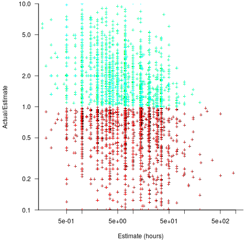
To experiment using these two packages I used the SiP dataset, which includes summary text for each task, and I have previously analysed the estimation task data.

The stm package:

The textProcessor function handles all the details of converting a vector of strings (e.g., summary text) to internal form (i.e., handling conversion to lower case, removing stop words, stemming, etc).

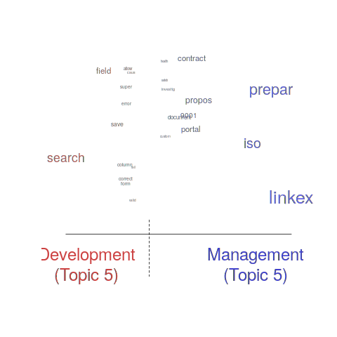
One of the input variables to the LDA process is the number of topics to use. Picking this value is something of a black art, and various functions are available for calculating and displaying concepts such as topic semantic coherence and exclusivity, the most commonly used words associated with a topic, and the documents in which these topics occur. Deciding the extent to which 10 or 15 topics produced the best results (values that sounded like a good idea to me) required domain knowledge that I did not have. The plot below shows the extent to which the words in topic 5 were associated with the Category column having the value “Development” or “Management” (code+data):

The psychtm package:

The prep_docs function is not as polished as the equivalent stm function, but the package’s first release was just last year.

After the data has been prepared, the call to fit a regression model that includes the LDA extracted topics is straightforward:

sip_topic_mod=gibbs_sldax(log(HoursActual) ~ log(HoursEstimate), data = cl_info,
                         docs = docs_vocab$documents, model = "sldax",
                         K = 10 # number of topics)

where: log(HoursActual) ~ log(HoursEstimate) is the simplest model fitted in the original analysis.

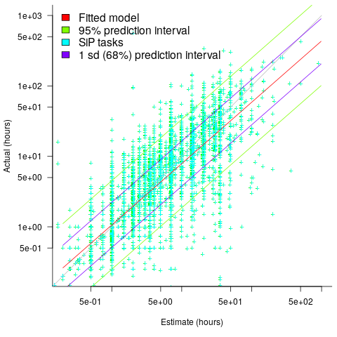
The fitted model had the form: , with the calculated coefficient for some topics not being significant. The value is close to that fitted in the original model. The value of is the fraction of the calculated to be present in the Summary text of the corresponding task.

I’m please to see that a regression model can be improved by adding topics derived from the Summary text.

The SiP data includes other information such as work Category (e.g., development, management), ProjectCode and DeveloperId. It is to be expected that these factors will have some impact on the words appearing in a task Summary, and hence the topics (the stm analysis showed this effect for Category).

When the model formula is changed to: log(HoursActual) ~ log(HoursEstimate)+ProjectCode, the quality of fit for most topics became very poor. Is this because ProjectCode and topics conveyed very similar information, or did I need to be more sophisticated when extracting topic models? This needs further investigation.

Can topic models be used to build prediction models?

Summary text can only be used to make predictions if it is available before the event being predicted, e.g., available before a task is completed and the actual effort is known.

My own habit is to update, or even create Summary text once a task is complete. I asked Stephen Cullen, my co-author on the original analysis and author of many of the Summary texts, about the process of creating the SiP Summary sentences. His reply was that the Summary field was an active document that was updated over time. I suspect the same is true for many task descriptions.

Not all estimation data includes as much information as the SiP dataset. If Summary text is one of the few pieces of information available, it may be possible to use it as a proxy for missing columns.

Perhaps it is possible to extract information from the SiP Summary text that is not also contained in the other recorded information. Having been successful this far, I will continue to investigate.