Derek Jones from The Shape of Code
This blog is moving to a new’ish domain (shape-of-code.com), and hosting company (HostGator). The existing url (shape-of-code.coding-guidelines.com) will continue to work for at least a year, and probably longer.
A beta version of the new site is now running. If things check out (please let me know if you see any issues), https://shape-of-code.com will become the official home next weekend, and the DNS entry for shape-of-code.coding-guidelines.com will be changed to point to the new address.
The existing coding-guidelines.com website has been hosted by PowWeb since June 2005. These days few people will have heard of PowWeb, but in 2005 they often appeared in the list of top hosting sites. I have had a few problems over the years, but I suspect nothing that I would have experienced from other providers. Over time, the functionality provided by PowWeb has decreased, compared to what they used to offer and what others offer today. But since my site usage has been essentially hosting a blog, I have not had a reason to move.
While I have had a nagging feeling I ought to move to a major provider, it was not until a post caused the site to be taken off-line because of a page-views per-hour limit being exceeded, that I decided to move. The limit was exceeded because an article appeared on news.ycombinator and became more popular, more rapidly, than my previous article appearances on ycombinator (which have topped out at 20K+ hits). Customer support were very responsive and quickly reset the page counter, once I contacted them and explained the situation. But why didn’t they inform me (I rarely hear from them, apart from billing, and one false alarm about the site sending spam), and why no option to upgrade?
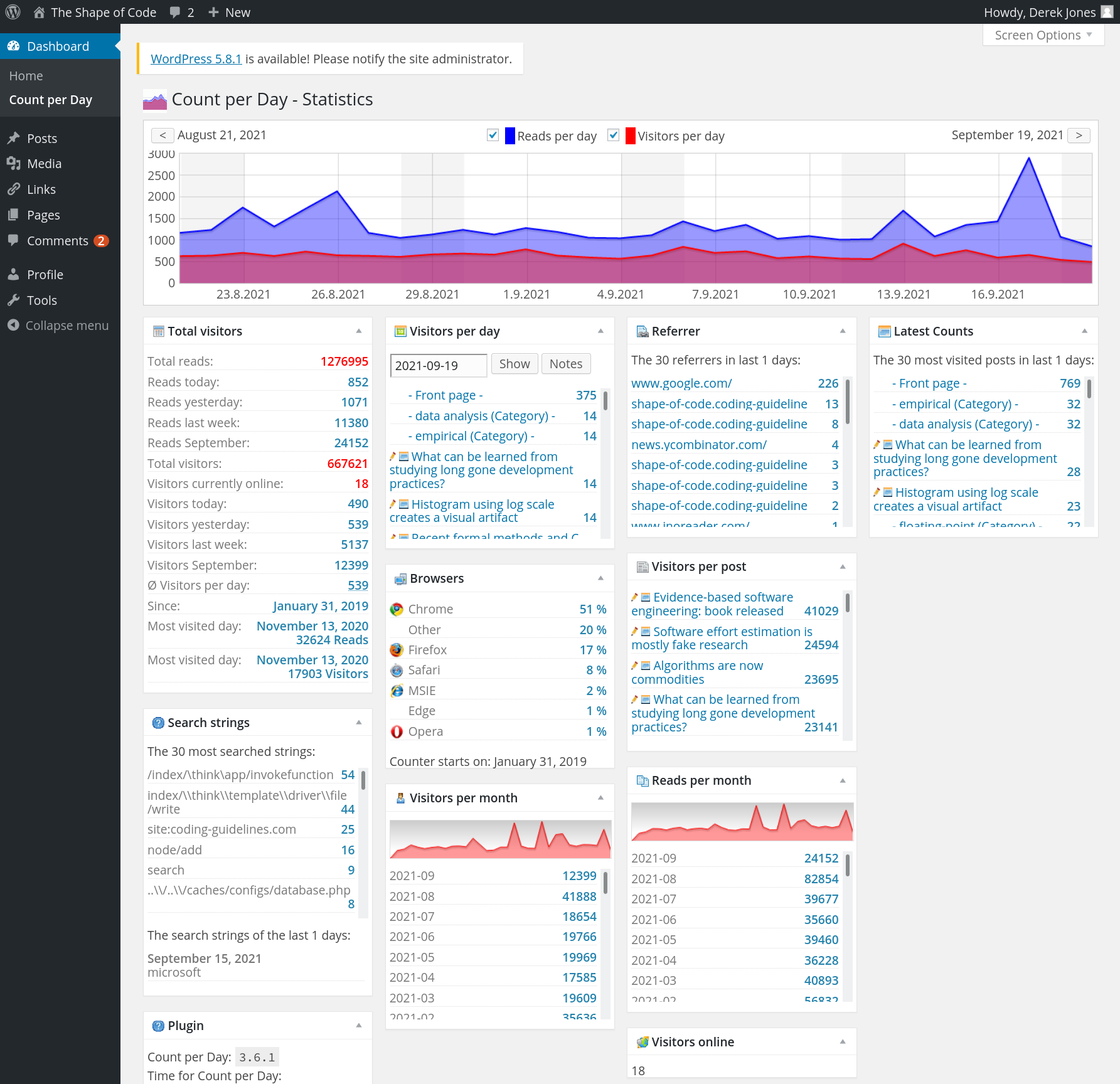
The screenshot below shows that the daily traffic is around 1K views (mostly from Google searches), with 20k+ daily peak views every few months (sometimes months after the article was posted):

Eight months later, the annual fee is due; time for action. HostGator is highly rated by many hosting reviews, and offered site migration (never having migrated a website before, I did not know it was essentially ftp’ing the contents, and maybe some basic WordPress stuff). I signed up.
As you may have guessed, my approach to website maintenance is: If it’s not broken, don’t fix it. This meant the site was running the oldest version of WordPress (4.2.30) and PHP (5.2, which reached end-of-life 10 years ago) that PowWeb supported.
As I learned about website and WordPress migration, I thought: I can do that. My Plan B was to get HostGator to do it.
WordPress migration turned out to be straight forward:
- export blog contents. WordPress generates an xml file,
- edit the xml file, replacing all occurrences of
shape-of-code.coding-guidelines.combyshape-of-code.com, - create WordPress blog on HostGator (to minimise the chance of incompatibilities I stayed with version 4, HostGator offers 4.9.18), selected a few options, and installed a few basic add-ons,
- ftp directories containing images and code+data to new site,
- import contents of xml file (there is a 512M limit, my file was 5.5M).
It worked 
I was not happy with the theme visually closest to the current blog (Twenty Sixteen), so I tried installing the existing theme (iNove). Despite not being maintained for eight years, it works well enough for me to decide to run with it.
I’m hoping that the new site will run with minimal input from me (apart from writing articles) for the next 10-years.

 , where
  is the mean length.
 , where
  is the mean length.
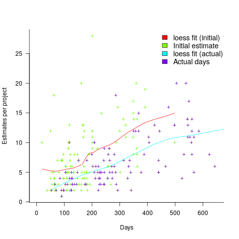
 ; the y-axis uses a log scale so that under/over estimates appear symmetrical (
 , and
, and  .
. (plotted in red). The top of the ‘cone’ does not represent managements’ increasing certainty, with project progress, it represents the mathematical upper bound on the possible inaccuracy of an estimate.
 ; the y-axis uses a log scale so that under/over estimates appear symmetrical (
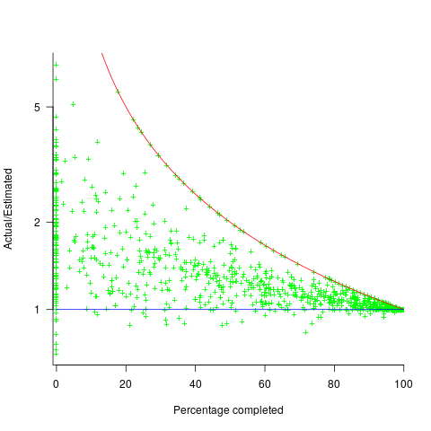
 , and
, and  .
. (plotted in red). The top of the ‘cone’ does not represent managements’ increasing certainty, with project progress, it represents the mathematical upper bound on the possible inaccuracy of an estimate.